Unit 1
State & explain Law of demand with the help of a schedule and a diagram.
The Law of Demand states that, when price of a commodity increases then demand of that commodity decreases and when price of a commodity decreases then demand decreases, other things remaining constant like income of the consumer, taste and preference of consumer etc.
This relationship between price and quantity demanded can be illustrated through a demand schedule and a demand curve.
Demand Schedule:
| Price (₹) | Quantity Demanded |
| 10 | 50 |
| 8 | 70 |
| 6 | 90 |
| 4 | 110 |
| 2 | 130 |
As the price decreases from ₹10 to ₹2, the quantity demanded increases, reflecting the inverse relationship.
Demand Curve:
In the demand curve diagram, the vertical axis represents the price, and the horizontal axis represents the quantity demanded. The demand curve typically slopes downward from left to right, indicating the negative relationship between price and quantity demanded.

This graphical representation visually demonstrates the Law of Demand, showcasing the tendency for consumers to buy more of a good as its price decreases and buy less as its price increases.
What is demand function? Explain the various factors determining the demand of a commodity.
A demand function represents the relationship between the quantity demanded of a good and the factors that influence that quantity.
It is typically expressed as Q = f(P, I, T, Pr, O), where:
Q is the quantity demanded,
P is the price of the good,
I is the consumer’s income,
T is the taste or preference of the consumer,
is the price of related goods (substitutes or complements),
O is other factors affecting demand.
Factors Determining Demand:
1. Price of the Good (P): The law of demand states that, all else being equal, as the price of a good increases, the quantity demanded decreases, and vice versa.
2. Consumer Income (I): Generally, as income rises, the demand for normal goods increases. For inferior goods, the opposite is true.
3. Tastes and Preferences (T): Consumer preferences heavily influence demand. Changes in fashion, trends, or cultural preferences can significantly impact the demand for certain goods.
4. Prices of Related Goods (Pr): The prices of substitutes and complements affect demand. If the price of a substitute increases, the demand for the original good may increase. Conversely, if the price of a complement increases, the demand for the original good may decrease.
5. Consumer Expectations (Ps): Anticipated future prices can influence current demand. If consumers expect prices to rise in the future, they may increase their current demand to avoid higher costs later.
6. Other Factors (O): Various factors like demographics, advertising, seasonality, and external shocks can influence demand. For example, a sudden health trend might increase the demand for organic foods.
Understanding these factors allows businesses and policymakers to make informed decisions about pricing, marketing, and resource allocation based on the expected behavior of consumers in the market. The demand function provides a mathematical representation of these relationships.
Contraction of Demand
Contraction of Demand means there is a decrease in the quantity demanded of the commodity due to an increase in its price.
Expansion of Demand
Expansion of Demand means there is an increase in the quantity demanded of the commodity due to a decrease in its price.
Increase in Demand
Increase in demand refers to an increase in the quantity demanded of quantity due to not because of change in its price but because of an increase in other factors like income of the consumer, change in the prices of substitutes and compliments and probably due to the change in taste and preference of the consumer.
Decrease in Demand
Decrease in demand refers to a decrease in the quantity demanded of quantity due to not because of change in its price but because of a decrease in other factors like income of the consumer, change in the prices of substitutes and compliments and probably due to the change in taste and preference of the consumer.

Elasticity of Demand


Income Elasticity of Demand

State the law of supply.
Supply refers to different quantities of a good that A supplier is willing to sell at different prices during a given period of time.
Factors on which it depends-
Price, Demand and Cost of factor of production etc.


Unit 2
Cardinal Utility Theory
It’s a way of measuring the level of satisfaction a consumer receives after consuming goods or services. This satisfaction can be measured and expressed in quantitative numbers.
Cardinal utility measures economic value through imaginary units, called “utils”.
Ordinal Utility Theory
Ordinal utility theory is an economic theory that states that a consumer’s satisfaction from consuming goods or services cannot be measured in numbers. Instead, it can be arranged in order of preference.
Ordinal utility theory claims that it is only meaningful to ask which option is better than the other, but it is meaningless to ask how much better it is or how good it is.
Difference between Cardinal and Ordinal
| Cardinal Utility | Ordinal Utility |
| 1. Cardinal Utility is a utility that determines the satisfaction of a commodity used by an individual and can be supported with a numeric value. | 1. Ordinal Utility defines that satisfaction of user goods can be ranked in order of preference but cannot be evaluated numerically. |
| 2. Cardinal Utility evaluates objectively. | 2. Ordinal Utility measures the utility of goods subjectively. |
| 3. Cardinal Utility is not much realistic as compared to the Ordinal Utility as quantitative evaluation of utility is not practicable. | 3. Ordinal Utility depends on qualitative measurement, which makes it more realistic. |
| 4. Cardinal Utility is based on indifference curve analysis. | 4. Ordinal Utility is based on marginal utility evaluation. |
Indifference Curves
The indifference curve are a study of consumer behavior based on the concept of ordinary utility analytics given by Professor Hicks and Allen. An indifference curve is a curve which shows different combinations of two goods capable of giving the consumer same level of satisfaction. Since the consumer gets the same satisfaction, he is therefore indifferent between them.
Assumptions
1. The consumer is a rational human being possessing full information.
2. The consumer can rank According to the satisfaction of he recives. For example. If there are combination of goods A,B,C. He can say that he prefers A to B or B to C.
3. The consumer is consistent with his behavior i.e if he prefers A to b B to C, then he will also prefer A to C
4. The consumer will always prefer a longer amount of goods that they smaller Amount.
| Combination | X | Y | MRS (Marginal Rate of Substitution ) |
| A | 1 | 12 | 4 |
| B | 2 | 8 | 2 |
| C | 3 | 6 | 1 |
| D | 4 | 5 |
The above table shows different combinations of the two goods X&Y giving same amount of satisfaction to the consumer.
Properties of Indifference Curve.
1. An indifference curve always slope downwards from left to right.

This is because when the amount of one commodity is increased, then the amount of the other good must be reduced. So that the level of satisfaction remains the same.
An indifference curve cannot be a horizontal straight line because different combinations will have same amount of Y but more amount of X. And therefore, will give different level of satisfaction.

Similarly, indifference curve cannot be a vertical straight line because it will have Same amount of X and more amount of Y.

Similarly, an Indifference curve cannot be upright sloping curve because there will be more combination of commodity of X&Y.

2. Indifference curves are convex to the origin.
A concave indifference curve will have increased Marginal Rate of Substitution (MRS) and straight-line indifference curve constant MRS.
3. No indifference curve can intersect with each other.
Two indifference curves cannot represent the same level of satisfaction, they cannot intersect each other.

4. Higher the indifference curve, higher the satisfaction.
Because the higher indifference curve will have combinations more of X as well as more of Y.
What do you mean by Consumers Equilibrium ? Explain with the help of indifference curve.
A consumer is said to be an equilibrium when he is buying such a combination of goods, which leaves him with no tendency to rearrange his purchases of goods. At the equilibrium point, the consumer satisfaction is maximized.
This can be explained with the help of following diagram.

Assumptions
1. The consumer has a given indifference map showing his preference for the two goods X&Y.
2. He has a fixed amount of income.
3. The prices of both the goods are given.
On the basis of the above assumptions, the budget line or the price line has been drawn as PL. IC1, IC2, IC3, IC4 are the different indifference curve showing the consumers preference. Various combination of A,B,C,D,E are all possible for the consumer to buy. The consumer will be at equilibrium at E on IC3 by OM amount of X and OR amount of Y. Other combinations like A & B , C& D will not be preferred by the consumer as they are on lower IC.
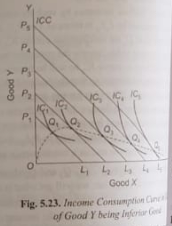
Income Effect
The income effect tries to measure changes in the consumers purchase of X & Y as a result of a change in his money income. P¹L¹,P²L²,P³L³,P⁴L⁴ are the different price lines showing an increase in the consumers money income. IC1, IC2, IC3 and IC4 are different indifference curve showing the consumers equlibrium at different levels. Q¹, Q², Q³, Q⁴ are different equilibrium point showing the Income Consumption Curve ( ICC).
For Example – The consumer was initially buying OM1 quantity of X and ON1 amount of Y. But when his income increased, he is now buying OM2 amount of X and ON2 amount of Y.


Substitution Effect
Substitution effect tries to measure the change in consumer purchase of X & Y as a result of a change in relative prices alone, real income remaining constant.
When the price of the commodity falls, real income of purchasing power of the consumer changes to keep the real income constant. So that the effect relative price change alone can be measure, price change is compensated by reducing the money income of the consumer.
There are two versions of the substitution effect, one by Hicks and Allen and other one Slutesky.
In Hicks and Allen approach, price change is accompanied by so much change in the money income that the consumer is neither better nor worse than before. In other words, the consumer satisfaction remains the same, or he is on the same indifference curve.
The amount by which the consumer money income has changed is known as the compensating variation in income.
This can be explained with the help of the following diagram.

PL is the original Priceline.
PL¹ is the new Priceline after a fall in the price of X.
The consumer was initially at equilibrium at point Q by OM amount of X & ON amount of Y.
AB is the price line which has been drawn to reduce this money income by so much that the consumer satisfaction is at the same level or on the same indifference curve.
Therefore, the consumer now is at equilibrium T by OM¹ of X & ON¹ of Y. So, M1 is the extra amount of X the consumer is buying now or substituting X for Y.
Price Effect
The price effect tries to measure the consumers changes in the price of a commodity when no compensating variation in income is made. In other words, price effect tries to show the increase in consumers purchase of a commodity as a result of a fall in the price of the commodity.

In the given diagram, PL, PL1, PL2 are different price line drawn showing a fall in the price of X.
The consumer’s equilibrium was initially at E by OM quantity of X and ON quantity of Y.
With subsequent fall in the price of X, the consumer is now buying more of X, which can be seen from the equilibrium points from E2, E3 buying now OM1 of X and further OM2 of X.
Revealed Preference Hypothesis
Reveal preference hypothesis put forward by Professor Samuelson, seeks to explain consumers demand based on his ‘actual behavior’. This theory is therefore based on behavioristic explanation of consumer demand.
According to this hypothesis, when the consumer is observed to choose a particular combination ‘A’ out of various other alternatives combination open to it, he then ‘reveals’ his preference for A over to the other combinations. In other words, he rejects the other combination and chooses ‘A’. His choice of a reveals his preference for ‘A’
This can be explained graphically.

PL is the Priceline.
Combination A, B, C on the price line are possible for consumer for buy.
The combination inside the triangle POL are considered to be inferior combinations which the consumer will not buy as they have less of X & Y.
Combination outside the price line marked by TAS are superior combinations, but which the consumer cannot afford to buy.
Combinations between PAT is not sure to the consumer as it can have more of Y but the amount of X is not more.
Similarly, combination between SAL can also be considered as Ignorance zone as here it has more of X but the quantity of Y is not known.
Therefore, by choosing A over all other combinations, revealed his preference for A.

Unit 3
What is production function ?
It is a mathematical relationship which shows the maximum output that can be produced with a given amount of input.
1. Short run production function.
In these changes in output is studied by keeping one factor fixed and changing the quantity of the variable factor.
This is because in short run fixed factors cannot be changed and output can be increased by varying only the variable factor.
Law of diminishing marginal returns and law of variable proportion is an example of short run production function.
The law of variable proportion states that as the quantity of one variable factor is increased with the fix factor, total product initially increases at an increasing rate, then diminishing rate and then starts to decrease.

2. Long run production function.
It studies to relationship between input and output when all factors of production can be changed simultaneously and in the same proportion.
In the long run, there are no fixed factors as all factors can be varied.
Return to scale is an example which may be studied in the following three ways.
A. Constant return to scale.
If input are increased in a given proportion and if output increases in the same proportion, then it is an example of constant return to scale.
Example.
If input increases by 10% and if output increases by 10%, then it is an example of constant returns to scale.
B. Increase in returns to scale.
If inputs are increased by a certain proportion, and if output increases more than that, then it is a case of increasing returns to scale.
Example.
When input increases by 10%, if output increases by more than 10%.
C. Decreasing returns to scale.
When input is increased by 10% but output is increased by less than 10%.
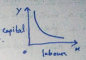
What are iso-quants? What are the properties of iso-quants?
It is the study of a production function with two factors regulated.
An isoquant is a curve which shows different combination of two functions capable of producing the same level of output.
Also called iso-product curve.


Properties of isoquants.
1. Isoquant slope downward from left to right.
This is because when the quantity of one factor is increased, the quantity of the other factor has to be decrease so that output remains constant.
2. No two isoquant can insert intersect each other.
This is because as soon in the given diagram there are two isoquants IQ1 and IQ2 intersecting at point P. On IQ1 A is equal to P on IQ2 B is equal to P. But A is not equal to be B as B is on a higher isoquant compared to A.

3. A normal isoquant always convex to the origin.
This is because of diminishing marginal rate of technical substitution.
Diminishing marginal rate of technical substitution implied that when the quantity of one factor is increased, less and less quantity of other factor will be substituted.
If isoquants are concave then it shows increasing marginal rate of technical substitution.
A straight line isoquant has constant rate of technical substitution.

4. Higher the isoquant higher the level of output.
This is because a higher isoquant will have more of labour as well as more of capital, and therefore will be able to produce a higher level of output.


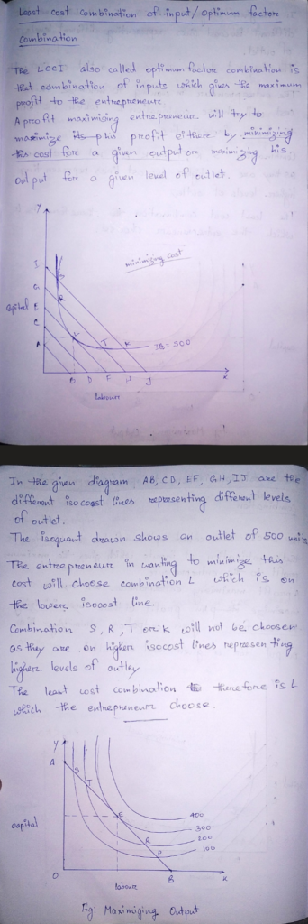

Implicit and Explicit cost of production ? Explain with the help of examples .
Implicit cost are the imputed values of cost for factor resources, which belongs to the entrepreneur himself.
Example. Salary of the managers or managerial duty ,interest on its own capital, rent for his own factory building.
Explicit costs are those cost of production for which the entrepreneur has to make a payment for it, and these are therefore recorded in the accounting books. This is also known as accounting cost of production.
Explicit Costs:
Explicit costs are the direct, tangible expenses a firm incurs in the production of goods or services. These costs involve actual cash outflows, and they are easily traceable and quantifiable. Examples of explicit costs include:
1. Raw Materials: The cost of materials directly used in the production process.
2. Labor Costs: Wages and salaries paid to employees.
3. Rent: The cost of leasing or renting production facilities.
4. Utilities: Expenses related to electricity, water, and other essential services for production.
Implicit Costs:
Implicit costs, on the other hand, are opportunity costs that don’t involve a direct cash outflow but represent the value of resources used in the production process. These costs are often related to the use of the owner’s resources or the potential income that could have been earned in alternative activities. Examples of implicit costs include:
1. Owner’s Time: If the owner of a business is actively involved in its operation, the value of their time devoted to the business is an implicit cost.
2. Opportunity Cost of Capital: The potential return that could have been earned if the funds invested in the business were used elsewhere.
3. Unpaid Family Labor: If family members contribute to the business without receiving a salary, the value of their labor represents an implicit cost.
Example: Consider a small bakery:
Explicit Costs: Flour, sugar, labor wages, rent for the bakery space, and electricity bills.
Implicit Costs: The owner’s time spent managing the bakery instead of pursuing a higher-paying job, the opportunity cost of the funds invested in the bakery instead of other ventures, and any family labor not compensated.
Understanding both explicit and implicit costs is crucial for a comprehensive analysis of a firm’s total economic cost. Explicit costs are recorded in accounting statements, while implicit costs often require a more nuanced economic perspective.
Economies of Scale
Economies of scale are cost advantages that companies gain when they increase production.
This happens because production costs can be spread over a larger number of goods.
Economies of scale are measured by the amount of output produced per unit of time. As the quantity of output produced increases, the per-unit fixed cost decreases.
There are two main types of economies of scale: internal and external.
Internal economies are controllable by management because they are internal to the company.
External economies depend upon external factors, such as the industry, geographic location, or government.
For example, car manufacturers can choose to expand their line of hybrid cars or increase the production of their existing lines of hybrid cars. This can lower their overall average cost of production because of the tax break incentive.
Economies of Scope
Economies of scope is an economic principle that states that a business’s unit cost to produce a product will decline as the variety of its products increases.
In other words, the more different-but-similar goods a business produces, the lower the total cost to produce each one will be.
Economies of scope occur when producing a wider variety of goods or services in tandem is more cost effective for a firm than producing less of a variety, or producing each good independently.
For example, a gas station that sells gasoline can sell soda, milk, baked goods, etc..
Another example of economies of scope is rail transportation. A single train can carry both passengers and freight more cheaply than having separate trains for passengers and for freight
Cost Function

Traditional Theory of Cost
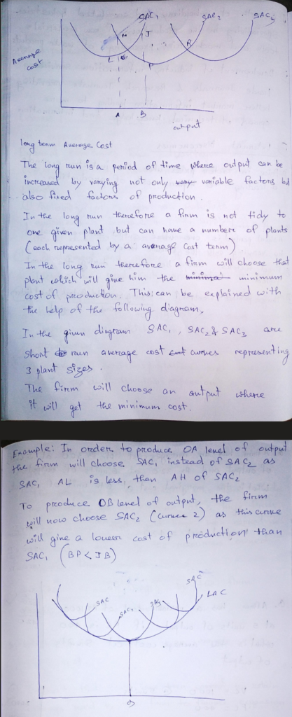
Modern Theory of Cost

Unit 4
Theory of Firm and Market Organisation :
Perfect Competition
Perfect competition is a type of market structure where there are a large number of buyers and sellers each selling a product which is exactly identical at a single price.
Perfect competition is also characterized by perfect knowledge between the buyers and sellers about the market conditions and there is also free entry and exit the firms.
Price under perfect competition is determined by aggregate demand and aggregate supply in the industry.
Every seller under perfect competition takes these prise as given and sales as many quantities as he can.
No individual seller can change this price. so price under perfect competition is always equal to p= AR = MR.
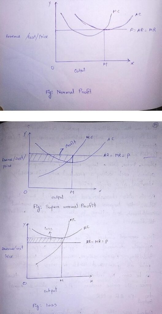
Output in perfect competition is determined at the point marginal revenue MR is equal to marginal cost MC.
Every individual seller will keep on producing so long as the revenue generated from the additional unit is greater than the cost. It will stop producing at a point where marginal revenue MR = marginal cost MC.
In the short run a firm under perfect competition can either make losses, supernormal profit or normal profit depending on the cost of production.
But in the long run every firm under perfect competition will be earning only normal profit. This is because when existing firms earn super normal profits new firms attracted by these profits will enter the industry. When this happens total output or supply will increase and if demand remains the same price or average revenue will come down to point of the average cost where all the firms will then be earning normal profit.
Similarly if firms were making losses they will exit the industry causing a contraction of the total supply or output.
When supply falls it will cause an increase in the price or the average revenue of the firms which then will make all firms or only normal profit.
Monopoly
Monopoly refers to market structure where there is a single seller for a product which has no close substitutes.
Also under a monopoly type of market there are restrictions or strong barriers to entry.
How is price and output determined under monopolistic market ?
A monopolist determines his price on the basis of the market demand curve which shows the different quantities consumers are willing to buy at different prices.
The average revenue curve or the demand curve facing a monopolist is downward sloping which indicates if the price is high the monopolist will be able to sell a smaller quantity. In other words he has to reduce the price in order to sell more.
The MR curve of the monopolist is also therefore downward sloping. Indicating that additional units will have to be sold at the reduced prices.
The MR curve is always less than the AR curve.
The output of the monopolist is also determined at the point where MR =MC .
Depending on his AC curve monopolist can either make Super normal profit or Normal Profit or even loses.


What do you mean by Price Discrimination ?
Price discrimination refers to the practice of selling the same product at different prices to different buyers.
Example: if a seller sells a refrigerator at 10,000 to one buyer and 12,000 to another buyer He is practicing price discrimination (all conditions of sale and delivery being the same)
Price discrimination may be –
a. Personal
Price discrimination is personal when a seller charges different prices from different persons
b. Local
Price discrimination is local when the seller charges different prices from different areas or localities.
c. According to use or trade
Price discrimination according to use or trade is when different prices are charged according to the use which is being put into.
When is Price Discrimination possible or profitable ?
Two fundamental conditions have to be present for making price discrimination possible –
1. price discrimination can occur only when it is not possible to transfer any unit of the product from one market to another or in other words product sold in a cheaper market cannot be sold in the dearer market.
2. price discrimination occurred when the buyers in the dearer market should not be able to transfer themselves to the cheaper market for buying the product.
Conditions Necessary for PD to be possible
Price discrimination is possible only in the following cases
a. nature of the commodity or the service is such that there is no possible of transference from one market to another.
Example in case of scale of direct services like that of a surgeon or a lawyer where the patient cannot pretend to be a poorer person to pay a small fee than a richer person
Monopolistic Competition
Monopolistic competition refers to a form of market structure where there are large number of firms producing similar products but which are not identical.
Under monopolistic competition, there are large number of firm producing differentiated products which are a close substitute for one another.
Features of monopolistic competition.
1. Large number of firms, each occupying a small share of the total market demand. Because of the numbers being large, there is stiff competition between them.
2. Product differentiation.
Products are not identical, though similar. Products are differentiated on the basis of actual or real differences or artificial differences.
3. Some influence over the price
Every firm under Monopolistic competition has got some influence in determining the price.
If a firm lower its price, it may be able to increase its demand.
On the other hand, if it increases the price of its product, it may lose some of its customers.
4. Non price competition.
Competition between firms under monopolistic competition is not so much on price, but more on advertisement, and other selling Cost.
5. Freedom to entry and exit.
Firms are free to enter and exit under monopolistic competition.
Product differentiation / Product variation
Productive differentiation is one of the most important feature of monopolistic competition.
Product in monopolistic competition are similar but not identical.
Seller differentiate their product on the basis of actual differences or imaginary differences.
Differentiation based on certain characteristics of the product itself such as exclusive painting feature trademark and trade names special types of packages or wraps any difference in quality design color or style.
Real qualitative differences like those of material design , like workmen ship or mean of differentiating product.
But imaginary differences created through advertising, use of attractive packets, trademarks and brand names are also common.
Excess capacity under Monopolistic Competition
One of the distinctive feature under monopolistic competition is the existence of excess capacity. Excess capacity refers to a situation where the equilibrium level of output is less than the socially optimum or ideal output. The socially level of output is generally considered to be the minimum point of the LAC.
The long run equilibrium output of firms under monopolistic competition is always at the following part of the average revenue curve.

Causes for excess capacity under monopolistic competition.
Excess capacity exist on a monopolistic competition because of two reasons.
1. The demand curve or the average revenue curve under monopolistic competition is downward sloping and as such it can be tangent only to the following portion of the long run average cost curve. A horizontal average revenue curve can be tangent to the minimum point of the LRC curve and hence it is only under perfect competition that there is no excess capacity.
2. Excess capacity exists under monopolistic competition because of the large number of firms each getting a very small share of the total market or demand. Therefore, it may not be required by the firm to produce at the socially optimum level of output.
Oligopoly
It is a type of market structure where there are few sellers selling products which may either be homogeneous or slightly differentiated.
Features or characteristics of oligopoly market.
1. Interdependence.
It is one of the most important features of oligopoly type of market. Because of the few firms in the industry, only decisions by one firm regarding price, output or the product will have a direct effect on the fortune of its rival firms, who will then retaliate similarly. For example. If one firm reduces its prices, other firm will also reduce their prices.
2. Importance of advertisement and selling cost.
The direct effect of interdependence between oligopolistic firm is that firm will have to employ various aggressive and defensive methods to gain a larger share of the market. In other words, competition between oligopolistic farm is not so much in price, but more on other factors like better advertisements and other selling and marketing techniques.
3. Group behavior.
Because of interdependence, it is noticed that firms under oligopolistic competition tends to follow common group policies or what is called common group behavior. Each farm will closely watch the behavior of other farms in taking any kind of decision.
Price and output decision under oligopolistic competition.
It has been observed that firms under oligopolistic market find it difficult to fix their price and output because of interdependence. An oligopolistic firm cannot assume that its rival firms will keep their prices at quantities constant when it made changes in its price or quantities when an oligopolistic firm changes its price, its rival firm will retaliate or react and also change their price which in turn would affect the demand of the former firm. Thus, an oligopolistic firm cannot have a sure and definitive demand curve, as its rival will also keep changing their prices. When an Oligopolist does not know his demand curve, he will therefore also not be able to fix his price and output.
However, various theories have been put forwarded by economists for explaining a price output model for oligopolistic market. The more popular version is that one given by the American economics name Sweezy.
According to Sweezy, ” The demand curve facing an oligopolist has a ” kink ” at the level of the revealing price. This is more famously known as the kinket DC hypothesis.
This hypothesis supports the view that there is “Price Rigidity” under oligopoly.
This can be explained with the help of the following diagram.
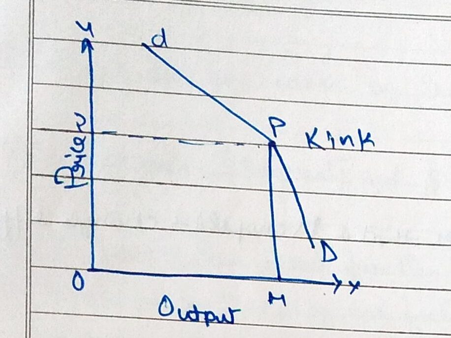
The small d is a DC facing an oligopoly.
The kink is formed at the prevailing price of P at upper segment of the DC.
dP is more elastic than the lower segment PD.
The price determinant is OP and the output is OM.
The price tends to be sticky at OP. This is because when the oligopolist lowers its price below the prevailing price, other competitor will also follow and hence he will not gain much. His demand curve will therefore will be more inelastic before the prevailing price.
On the other hand when he raises his price other competitors may not increase their prices which in turn will make him lose his customer. The DC therefore is more elastic on the upper segment of the prevailing price.
This shows that prices OM tends to be sticky or rigid at the point of the kink.